Poisson Regression: Modeling Tool Diversity Across Islands

Centering, correlations, and counterfactual posteriors in Oceanic tool kit evolution.

bayesian

regression

mcmc

statistics

Analyzes technological diversity across Oceanic island societies using Poisson regression with interaction terms. Shows how parameter centering reduces posterior correlation and how counterfactual predictions reveal contact effects masked by correlated parameters.

Published

May 21, 2025

%matplotlib inline
import numpy as np
import scipy as sp
import matplotlib as mpl
import matplotlib.cm as cm
import matplotlib.pyplot as plt
import pandas as pd
pd.set_option('display.width', 500)
pd.set_option('display.max_columns', 100)
pd.set_option('display.notebook_repr_html', True)
import seaborn as sns
sns.set_style("whitegrid")
sns.set_context("poster")
import pymc as pm
import arviz as az

From Mcelreath:

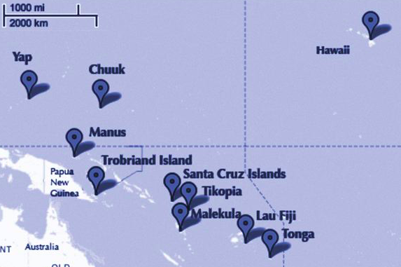
The island societies of Oceania provide a natural experiment in technological evolution. Different historical island populations possessed tool kits of different size. These kits include fish hooks, axes, boats, hand plows, and many other types of tools. A number of theories predict that larger populations will both develop and sustain more complex tool kits. So the natural variation in population size induced by natural variation in island size in Oceania provides a natural experiment to test these ideas. It’s also suggested that contact rates among populations effectively increase population size, as it’s relevant to technological evolution. So variation in contact rates among Oceanic societies is also relevant. (McElreath 313)

Map of the 10 Oceanic island societies in the Kline dataset [Source: McElreath, Statistical Rethinking]

Setting up the model and data

Some points to take into account:

sample size is not umber of rows, after all this is a count model
the data is small, so we will need regularizing to avoid overfitting
outcome will be total_tools which we will model as proportional to log(population) as theory says it depends on order of magnitude
number of tools incereases with contact rate
we will, over multiple attempts, be testing the idea that the impact of population on tool counts is increased by high contact. This is an example of an interaction. Specifically this is a positive interaction between log(population) and contact.

df=pd.read_csv("data/islands.csv", sep=';')
df

	culture	population	contact	total_tools	mean_TU
0	Malekula	1100	low	13	3.2
1	Tikopia	1500	low	22	4.7
2	Santa Cruz	3600	low	24	4.0
3	Yap	4791	high	43	5.0
4	Lau Fiji	7400	high	33	5.0
5	Trobriand	8000	high	19	4.0
6	Chuuk	9200	high	40	3.8
7	Manus	13000	low	28	6.6
8	Tonga	17500	high	55	5.4
9	Hawaii	275000	low	71	6.6

df['logpop']=np.log(df.population)
df['clevel']=(df.contact=='high')*1
df

	culture	population	contact	total_tools	mean_TU	logpop	clevel
0	Malekula	1100	low	13	3.2	7.003065	0
1	Tikopia	1500	low	22	4.7	7.313220	0
2	Santa Cruz	3600	low	24	4.0	8.188689	0
3	Yap	4791	high	43	5.0	8.474494	1
4	Lau Fiji	7400	high	33	5.0	8.909235	1
5	Trobriand	8000	high	19	4.0	8.987197	1
6	Chuuk	9200	high	40	3.8	9.126959	1
7	Manus	13000	low	28	6.6	9.472705	0
8	Tonga	17500	high	55	5.4	9.769956	1
9	Hawaii	275000	low	71	6.6	12.524526	0

Lets write down the model we plan to fit.

M1

\[ \begin{eqnarray} T_i & \sim & Poisson(\lambda_i)\\ log(\lambda_i) & = & \alpha + \beta_P log(P_i) + \beta_C C_i + \beta_{PC} C_i log(P_i)\\ \alpha & \sim & N(0,100)\\ \beta_P & \sim & N(0,1)\\ \beta_C & \sim & N(0,1)\\ \beta_{PC} & \sim & N(0,1) \end{eqnarray} \]

The \(\beta\)s have strongly regularizing priors on them, because the sample is small, while the \(\alpha\) prior is essentially a flat prior.

Implementation in pymc

import pytensor.tensor as pt
with pm.Model() as m1:
    betap = pm.Normal("betap", 0, 1)
    betac = pm.Normal("betac", 0, 1)
    betapc = pm.Normal("betapc", 0, 1)
    alpha = pm.Normal("alpha", 0, 100)
    loglam = alpha + betap*df.logpop + betac*df.clevel + betapc*df.clevel*df.logpop
    y = pm.Poisson("ntools", mu=pt.exp(loglam), observed=df.total_tools)

with m1:
    idata = pm.sample(10000, cores=2)

Initializing NUTS using jitter+adapt_diag...
Multiprocess sampling (2 chains in 2 jobs)
NUTS: [betap, betac, betapc, alpha]

/Users/rahul/Library/Caches/uv/archive-v0/aTiHGxSE8gD8G3bEQyxJO/lib/python3.14/site-packages/rich/live.py:260: 
UserWarning: install "ipywidgets" for Jupyter support
  warnings.warn('install "ipywidgets" for Jupyter support')

Sampling 2 chains for 1_000 tune and 10_000 draw iterations (2_000 + 20_000 draws total) took 11 seconds.
We recommend running at least 4 chains for robust computation of convergence diagnostics

az.summary(idata)

	mean	sd	hdi_3%	hdi_97%	mcse_mean	mcse_sd	ess_bulk	ess_tail	r_hat
betap	0.264	0.035	0.199	0.329	0.000	0.000	8004.0	7574.0	1.0
betac	-0.093	0.837	-1.683	1.468	0.010	0.008	6618.0	7068.0	1.0
betapc	0.043	0.092	-0.134	0.210	0.001	0.001	6637.0	7307.0	1.0
alpha	0.940	0.361	0.226	1.591	0.004	0.004	8030.0	7963.0	1.0

az.plot_trace(idata);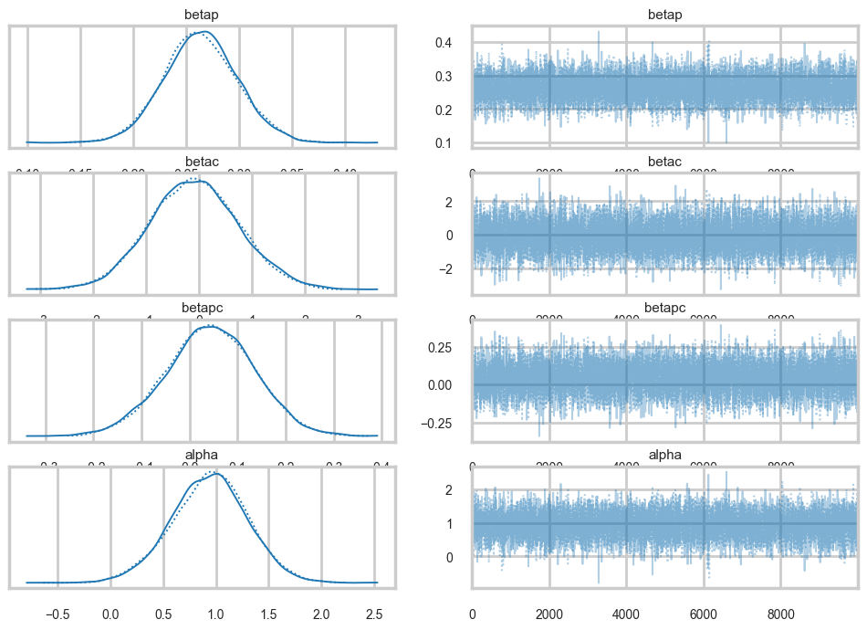

az.plot_autocorr(idata);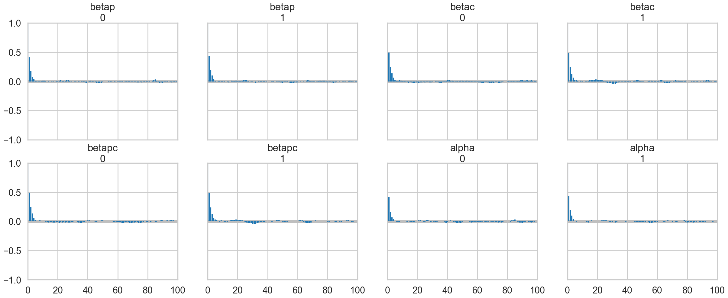

Our traces an autocorrelations look pretty good. pymc does quick work on the model

Posteriors

az.plot_posterior(idata);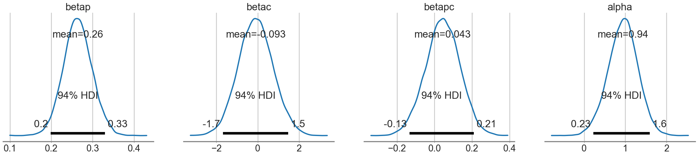

Looking at the posteriors reveals something interesting. The posterior for \(\beta_p\) is, as expected from theory, showing a positive effect. The posterior is fairly tightly constrained. The posteriors for \(\beta_c\) and \(\beta_{pc}\) both overlap 0 substantially, and seem comparatively poorly constrained.

At this point you might be willing to say that there is no substantial effect of contact rate, directly or through the interaction.

You would be wrong.

Posterior check with counterfactual predictions.

Lets get \(\lambda\) traces for high-contact and low contact

lamlow = lambda logpop: idata.posterior['alpha'].values.flatten() + idata.posterior['betap'].values.flatten() * logpop
lamhigh = lambda logpop: idata.posterior['alpha'].values.flatten() + (idata.posterior['betap'].values.flatten() + idata.posterior['betapc'].values.flatten()) * logpop + idata.posterior['betac'].values.flatten()

Now let us see what happens at an intermediate log(pop) of 8:

sns.histplot(lamhigh(8) - lamlow(8), kde=True);
plt.axvline(0);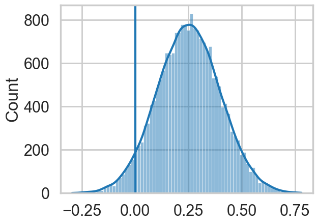

We can see evidence of a fairly strong positive effect of contact in this “counterfactual posterior”, with most of the weight above 0.

So what happened?

Posterior scatter plots

We make posterior scatter plots and this give us the answer.

def postscat(idata, thevars):
    d = {}
    for v in thevars:
        d[v] = idata.posterior[v].values.flatten()
    df = pd.DataFrame.from_dict(d)
    return sns.pairplot(df)

postscat(idata, ["betap", "betac", "betapc", "alpha"])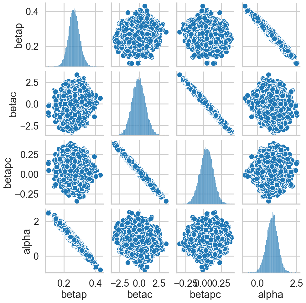

Look at the very strong negative correlations between \(\alpha\) and \(\beta_p\), and the very strong ones between \(\beta_c\) and \(\beta_{pc}\). The latter is the cause for the 0-overlaps. When \(\beta_c\) is high, \(\beta_{pc}\) must be low, and vice-versa. As a result, its not enough to observe just the marginal uncertainty of each parameter; you must look at the joint uncertainty of the correlated variables.

You would have seen that this might be a problem if you looked at \(n_{eff}\):

az.ess(idata)

Fixing by centering

As usual, centering the log-population fixes things:

df['logpop_c'] = df.logpop - df.logpop.mean()

with pm.Model() as m1c:
    betap = pm.Normal("betap", 0, 1)
    betac = pm.Normal("betac", 0, 1)
    betapc = pm.Normal("betapc", 0, 1)
    alpha = pm.Normal("alpha", 0, 100)
    loglam = alpha + betap*df['logpop_c'] + betac*df.clevel + betapc*df.clevel*df['logpop_c']
    y = pm.Poisson("ntools", mu=pt.exp(loglam), observed=df.total_tools)

with m1c:
    idata1c = pm.sample(10000, cores=2)

Initializing NUTS using jitter+adapt_diag...
Multiprocess sampling (2 chains in 2 jobs)
NUTS: [betap, betac, betapc, alpha]

/Users/rahul/Library/Caches/uv/archive-v0/aTiHGxSE8gD8G3bEQyxJO/lib/python3.14/site-packages/rich/live.py:260: 
UserWarning: install "ipywidgets" for Jupyter support
  warnings.warn('install "ipywidgets" for Jupyter support')

Sampling 2 chains for 1_000 tune and 10_000 draw iterations (2_000 + 20_000 draws total) took 2 seconds.
We recommend running at least 4 chains for robust computation of convergence diagnostics

az.ess(idata1c)

az.summary(idata1c)

	mean	sd	hdi_3%	hdi_97%	mcse_mean	mcse_sd	ess_bulk	ess_tail	r_hat
betap	0.263	0.035	0.199	0.330	0.000	0.000	14664.0	14588.0	1.0
betac	0.284	0.116	0.071	0.508	0.001	0.001	13651.0	13802.0	1.0
betapc	0.068	0.171	-0.252	0.388	0.001	0.001	15763.0	13145.0	1.0
alpha	3.312	0.089	3.143	3.477	0.001	0.001	13521.0	12501.0	1.0

postscat(idata1c, ["betap", "betac", "betapc", "alpha"])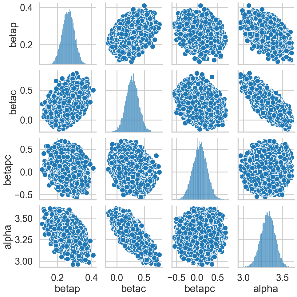

az.plot_posterior(idata1c);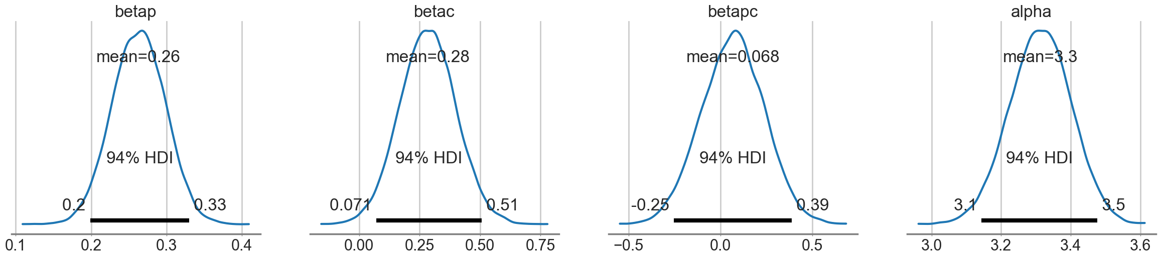

How do we decide whether the interaction is significant or not? We’ll use model comparison to achieve this!