Geographic Correlation and Oceanic Tools

Gaussian process covariance captures spatial correlation between island societies.

bayesian

regression

gaussian-processes

models

We extend the oceanic tools Poisson regression with a custom GP covariance matrix that models geographic correlation between societies. The inverse-square distance kernel reveals how nearby islands share tool-making knowledge.

Published

May 28, 2025

We read back the Oceanic tools data with geographic coordinates and a distance matrix to model spatial correlation between island societies using a Gaussian Process covariance structure.

%matplotlib inline
import numpy as np
import scipy as sp
import matplotlib as mpl
import matplotlib.cm as cm
import matplotlib.pyplot as plt
import pandas as pd
pd.set_option('display.width', 500)
pd.set_option('display.max_columns', 100)
pd.set_option('display.notebook_repr_html', True)
import seaborn as sns
sns.set_style("whitegrid")
sns.set_context("poster")
import pymc as pm
import arviz as az

Reading in our data

We read back the Oceanic tools data

df = pd.read_csv("data/Kline2.csv", sep=';')
df.head()

	culture	population	contact	total_tools	mean_TU	lat	lon	lon2	logpop
0	Malekula	1100	low	13	3.2	-16.3	167.5	-12.5	7.003065
1	Tikopia	1500	low	22	4.7	-12.3	168.8	-11.2	7.313220
2	Santa Cruz	3600	low	24	4.0	-10.7	166.0	-14.0	8.188689
3	Yap	4791	high	43	5.0	9.5	138.1	-41.9	8.474494
4	Lau Fiji	7400	high	33	5.0	-17.7	178.1	-1.9	8.909235

And center it

df['logpop_c'] = df.logpop - df.logpop.mean()

df.head()

	culture	population	contact	total_tools	mean_TU	lat	lon	lon2	logpop	logpop_c
0	Malekula	1100	low	13	3.2	-16.3	167.5	-12.5	7.003065	-1.973939
1	Tikopia	1500	low	22	4.7	-12.3	168.8	-11.2	7.313220	-1.663784
2	Santa Cruz	3600	low	24	4.0	-10.7	166.0	-14.0	8.188689	-0.788316
3	Yap	4791	high	43	5.0	9.5	138.1	-41.9	8.474494	-0.502510
4	Lau Fiji	7400	high	33	5.0	-17.7	178.1	-1.9	8.909235	-0.067769

And read in the distance matrix

dfd = pd.read_csv("data/distmatrix.csv", header=None)
dij=dfd.values
dij

array([[0.   , 0.475, 0.631, 4.363, 1.234, 2.036, 3.178, 2.794, 1.86 ,
        5.678],
       [0.475, 0.   , 0.315, 4.173, 1.236, 2.007, 2.877, 2.67 , 1.965,
        5.283],
       [0.631, 0.315, 0.   , 3.859, 1.55 , 1.708, 2.588, 2.356, 2.279,
        5.401],
       [4.363, 4.173, 3.859, 0.   , 5.391, 2.462, 1.555, 1.616, 6.136,
        7.178],
       [1.234, 1.236, 1.55 , 5.391, 0.   , 3.219, 4.027, 3.906, 0.763,
        4.884],
       [2.036, 2.007, 1.708, 2.462, 3.219, 0.   , 1.801, 0.85 , 3.893,
        6.653],
       [3.178, 2.877, 2.588, 1.555, 4.027, 1.801, 0.   , 1.213, 4.789,
        5.787],
       [2.794, 2.67 , 2.356, 1.616, 3.906, 0.85 , 1.213, 0.   , 4.622,
        6.722],
       [1.86 , 1.965, 2.279, 6.136, 0.763, 3.893, 4.789, 4.622, 0.   ,
        5.037],
       [5.678, 5.283, 5.401, 7.178, 4.884, 6.653, 5.787, 6.722, 5.037,
        0.   ]])

Implementing the simple tools:logpop model and varying intercepts models

import pytensor.tensor as pt

with pm.Model() as m2c_onlyp:
    betap = pm.Normal("betap", 0, 1)
    alpha = pm.Normal("alpha", 0, 10)
    loglam = alpha + betap*df.logpop_c
    y = pm.Poisson("ntools", mu=pt.exp(loglam), observed=df.total_tools)
    trace2c_onlyp = pm.sample(6000, tune=1000)

Initializing NUTS using jitter+adapt_diag...
Multiprocess sampling (4 chains in 4 jobs)
NUTS: [betap, alpha]

/Users/rahul/Library/Caches/uv/archive-v0/aTiHGxSE8gD8G3bEQyxJO/lib/python3.14/site-packages/rich/live.py:260: 
UserWarning: install "ipywidgets" for Jupyter support
  warnings.warn('install "ipywidgets" for Jupyter support')

Sampling 4 chains for 1_000 tune and 6_000 draw iterations (4_000 + 24_000 draws total) took 2 seconds.

az.summary(trace2c_onlyp)

	mean	sd	hdi_3%	hdi_97%	mcse_mean	mcse_sd	ess_bulk	ess_tail	r_hat
betap	0.239	0.031	0.179	0.297	0.0	0.0	20521.0	16397.0	1.0
alpha	3.478	0.058	3.372	3.588	0.0	0.0	20922.0	16520.0	1.0

Notice that \(\beta_P\) has a value around 0.24

We also implement the varying intercepts per society model from before

with pm.Model() as m3c:
    betap = pm.Normal("betap", 0, 1)
    alpha = pm.Normal("alpha", 0, 10)
    sigmasoc = pm.HalfCauchy("sigmasoc", 1)
    alphasoc = pm.Normal("alphasoc", 0, sigmasoc, shape=df.shape[0])
    loglam = alpha + alphasoc + betap*df.logpop_c 
    y = pm.Poisson("ntools", mu=pt.exp(loglam), observed=df.total_tools)
with m3c:
    trace3 = pm.sample(6000, tune=1000, target_accept=0.95)

Initializing NUTS using jitter+adapt_diag...
Multiprocess sampling (4 chains in 4 jobs)
NUTS: [betap, alpha, sigmasoc, alphasoc]

/Users/rahul/Library/Caches/uv/archive-v0/aTiHGxSE8gD8G3bEQyxJO/lib/python3.14/site-packages/rich/live.py:260: 
UserWarning: install "ipywidgets" for Jupyter support
  warnings.warn('install "ipywidgets" for Jupyter support')

Sampling 4 chains for 1_000 tune and 6_000 draw iterations (4_000 + 24_000 draws total) took 5 seconds.
There were 10 divergences after tuning. Increase `target_accept` or reparameterize.

az.summary(trace3)

	mean	sd	hdi_3%	hdi_97%	mcse_mean	mcse_sd	ess_bulk	ess_tail	r_hat
betap	0.261	0.081	0.107	0.416	0.001	0.001	9947.0	9891.0	1.0
alpha	3.443	0.120	3.211	3.667	0.001	0.001	7646.0	8098.0	1.0
alphasoc[0]	-0.201	0.241	-0.665	0.243	0.002	0.002	12562.0	11942.0	1.0
alphasoc[1]	0.042	0.221	-0.367	0.478	0.002	0.002	11734.0	10870.0	1.0
alphasoc[2]	-0.048	0.195	-0.418	0.331	0.002	0.002	12818.0	12931.0	1.0
alphasoc[3]	0.325	0.189	-0.025	0.678	0.002	0.002	7467.0	9482.0	1.0
alphasoc[4]	0.044	0.176	-0.281	0.391	0.002	0.001	12480.0	11816.0	1.0
alphasoc[5]	-0.317	0.208	-0.713	0.049	0.002	0.002	11430.0	12974.0	1.0
alphasoc[6]	0.145	0.171	-0.169	0.478	0.002	0.001	11496.0	11783.0	1.0
alphasoc[7]	-0.171	0.182	-0.533	0.151	0.002	0.001	12357.0	13019.0	1.0
alphasoc[8]	0.274	0.175	-0.042	0.613	0.002	0.001	9749.0	10910.0	1.0
alphasoc[9]	-0.093	0.288	-0.651	0.458	0.003	0.003	10202.0	9662.0	1.0
sigmasoc	0.308	0.127	0.087	0.545	0.002	0.001	4838.0	3874.0	1.0

A model with a custom covariance matrix

The assumption here now is that the intercepts for these various societies are correlated…

We use a custom covariance matrix which inverse-square weights distance

GP covariance matrix: squared-exponential kernel weighted by geographic distance, plus a noise term

You have seen this before! This is an example of a Gaussian Process Covariance Matrix.

Here is the complete model:

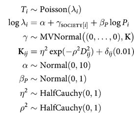
Full model specification: Poisson regression with GP-correlated society intercepts and distance-based covariance

with pm.Model() as mgc:
    betap = pm.Normal("betap", 0, 1)
    alpha = pm.Normal("alpha", 0, 10)
    etasq = pm.HalfCauchy("etasq", 1)
    rhosq = pm.HalfCauchy("rhosq", 1)
    means = pt.stack([0.0]*10)
    sigma_matrix = pt.diag(pt.as_tensor_variable([0.01]*10))
    cov = pt.exp(-rhosq*dij*dij)*etasq + sigma_matrix
    gammasoc = pm.MvNormal("gammasoc", means, cov=cov, shape=df.shape[0])
    loglam = alpha + gammasoc + betap*df.logpop_c 
    y = pm.Poisson("ntools", mu=pt.exp(loglam), observed=df.total_tools)

with mgc:
    mgctrace = pm.sample(10000, tune=2000, target_accept=0.95)

Initializing NUTS using jitter+adapt_diag...
Multiprocess sampling (4 chains in 4 jobs)
NUTS: [betap, alpha, etasq, rhosq, gammasoc]

/Users/rahul/Library/Caches/uv/archive-v0/aTiHGxSE8gD8G3bEQyxJO/lib/python3.14/site-packages/rich/live.py:260: 
UserWarning: install "ipywidgets" for Jupyter support
  warnings.warn('install "ipywidgets" for Jupyter support')

Sampling 4 chains for 2_000 tune and 10_000 draw iterations (8_000 + 40_000 draws total) took 42 seconds.

az.summary(mgctrace)

	mean	sd	hdi_3%	hdi_97%	mcse_mean	mcse_sd	ess_bulk	ess_tail	r_hat
betap	0.246	0.115	0.028	0.469	0.001	0.001	10228.0	11850.0	1.0
alpha	3.509	0.354	2.861	4.149	0.006	0.013	4779.0	3911.0	1.0
gammasoc[0]	-0.268	0.455	-1.121	0.549	0.007	0.012	5484.0	4869.0	1.0
gammasoc[1]	-0.120	0.443	-0.968	0.670	0.007	0.012	5099.0	4180.0	1.0
gammasoc[2]	-0.164	0.428	-0.982	0.587	0.007	0.012	5138.0	4151.0	1.0
gammasoc[3]	0.300	0.385	-0.414	0.991	0.006	0.012	5388.0	4369.0	1.0
gammasoc[4]	0.032	0.379	-0.660	0.720	0.006	0.013	5340.0	4222.0	1.0
gammasoc[5]	-0.454	0.388	-1.163	0.214	0.006	0.012	5582.0	4762.0	1.0
gammasoc[6]	0.102	0.374	-0.585	0.773	0.006	0.013	5442.0	4361.0	1.0
gammasoc[7]	-0.258	0.376	-0.952	0.402	0.006	0.013	5448.0	4625.0	1.0
gammasoc[8]	0.239	0.357	-0.391	0.908	0.005	0.013	5642.0	4511.0	1.0
gammasoc[9]	-0.115	0.460	-0.978	0.770	0.005	0.009	8816.0	8235.0	1.0
etasq	0.352	0.590	0.000	1.007	0.007	0.058	6572.0	9485.0	1.0
rhosq	2.028	61.589	0.002	3.745	0.361	28.788	7949.0	11599.0	1.0

az.plot_trace(mgctrace);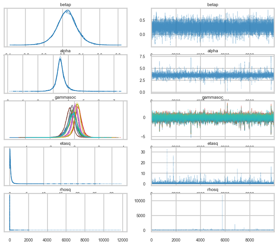

az.plot_autocorr(mgctrace);

/Users/rahul/Library/Caches/uv/archive-v0/aTiHGxSE8gD8G3bEQyxJO/lib/python3.14/site-packages/arviz/plots/plot_utils.py:270: UserWarning: rcParams['plot.max_subplots'] (40) is smaller than the number of variables to plot (56) in plot_autocorr, generating only 40 plots
  warnings.warn(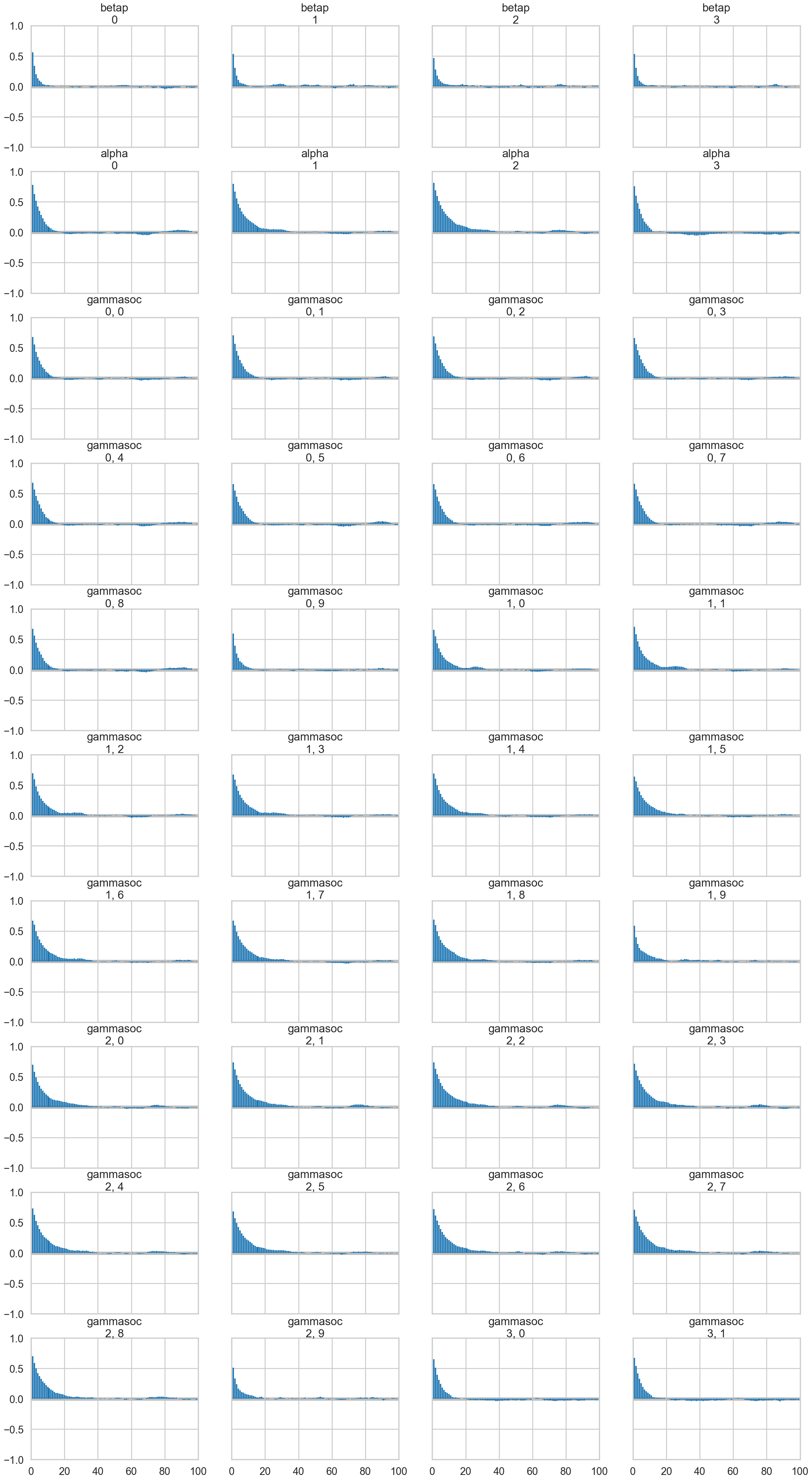

d={}
gammasoc_samples = mgctrace.posterior['gammasoc'].values.reshape(-1, 10)
for i, v in enumerate(df.culture.values):
    d[v] = gammasoc_samples[:,i]
dfsamps=pd.DataFrame.from_dict(d)
dfsamps.head()

	Malekula	Tikopia	Santa Cruz	Yap	Lau Fiji	Trobriand	Chuuk	Manus	Tonga	Hawaii
0	-0.130590	0.089298	-0.181058	0.615596	0.044638	0.310527	0.318529	0.011540	0.522527	0.314769
1	-0.086934	0.260856	-0.154601	0.322845	0.349256	-0.795153	0.188721	-0.294910	0.368426	-0.112205
2	-0.032733	-0.008312	0.203633	0.255771	0.592531	-0.736068	0.244687	-0.314360	0.449234	-0.123681
3	-0.103811	-0.273942	0.047349	0.704714	0.157025	-0.358446	0.295830	0.189327	0.385959	0.165699
4	-0.138728	0.030216	-0.301498	0.259886	0.256591	-0.179903	0.237708	-0.223339	0.380631	0.238701

dfsamps.describe()

	Malekula	Tikopia	Santa Cruz	Yap	Lau Fiji	Trobriand	Chuuk	Manus	Tonga	Hawaii
count	40000.000000	40000.000000	40000.000000	40000.000000	40000.000000	40000.000000	40000.000000	40000.000000	40000.000000	40000.000000
mean	-0.267976	-0.119667	-0.164049	0.300261	0.031830	-0.453667	0.102345	-0.257916	0.238663	-0.115166
std	0.455163	0.443377	0.427740	0.384622	0.378590	0.388457	0.373908	0.376287	0.356762	0.459638
min	-5.289634	-4.423674	-4.465862	-3.658895	-3.881839	-4.573565	-3.968056	-4.391581	-3.535199	-4.035076
25%	-0.494601	-0.337898	-0.363096	0.115944	-0.143074	-0.637728	-0.066815	-0.431598	0.076133	-0.363911
50%	-0.236810	-0.093558	-0.132354	0.309491	0.046415	-0.418354	0.116564	-0.231101	0.248910	-0.108310
75%	-0.008959	0.128550	0.076217	0.503830	0.229287	-0.231597	0.297074	-0.055373	0.422726	0.138756
max	3.642086	3.495336	3.480449	3.841792	3.590994	2.914655	3.495762	3.064075	3.666528	3.068279

Plotting posteriors and predictives

Lets plot the covariance posteriors for the 100 random samples in the trace.

smalleta=np.random.choice(mgctrace.posterior['etasq'].values.flatten(), replace=False, size=100)
smallrho=np.random.choice(mgctrace.posterior['rhosq'].values.flatten(), replace=False, size=100)

with sns.plotting_context('poster'):
    d=np.linspace(0,10,100)
    for i in range(100):
        covarod = lambda d: smalleta[i]*np.exp(-smallrho[i]*d*d)
        plt.plot(d, covarod(d),alpha=0.1, color='k')
    medetasq=np.median(mgctrace.posterior['etasq'].values.flatten())
    medrhosq=np.median(mgctrace.posterior['rhosq'].values.flatten())
    covarodmed = lambda d: medetasq*np.exp(-medrhosq*d*d)
    plt.plot(d, covarodmed(d),alpha=1.0, color='k', lw=3)
    plt.ylim([0,1]);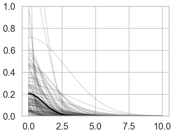

The x-axis is thousands of kilometers. Notice how almost everything damps out by 4000 kms. Lets calculate the median correlation matrix:

medkij = np.diag([0.01]*10)+medetasq*(np.exp(-medrhosq*dij*dij))

#from statsmodels
def cov2corr(cov, return_std=False):
    '''convert covariance matrix to correlation matrix

    Parameters
    ----------
    cov : array_like, 2d
        covariance matrix, see Notes

    Returns
    -------
    corr : ndarray (subclass)
        correlation matrix
    return_std : bool
        If this is true then the standard deviation is also returned.
        By default only the correlation matrix is returned.

    Notes
    -----
    This function does not convert subclasses of ndarrays. This requires
    that division is defined elementwise. np.ma.array and np.matrix are allowed.

    '''
    cov = np.asanyarray(cov)
    std_ = np.sqrt(np.diag(cov))
    corr = cov / np.outer(std_, std_)
    if return_std:
        return corr, std_
    else:
        return corr

medcorrij=cov2corr(medkij)
medcorrij

array([[1.00000000e+00, 8.69835262e-01, 8.11247323e-01, 4.34367364e-04,
        5.14947515e-01, 1.78423268e-01, 1.60816245e-02, 4.06297035e-02,
        2.35399591e-01, 2.09068998e-06],
       [8.69835262e-01, 1.00000000e+00, 9.15425265e-01, 8.36612901e-04,
        5.13920440e-01, 1.87081494e-01, 3.35913172e-02, 5.34275935e-02,
        2.00129903e-01, 1.20288892e-05],
       [8.11247323e-01, 9.15425265e-01, 1.00000000e+00, 2.31844903e-03,
        3.60868694e-01, 2.93087429e-01, 6.35978815e-02, 1.01103669e-01,
        1.16791052e-01, 7.22676264e-06],
       [4.34367364e-04, 8.36612901e-04, 2.31844903e-03, 1.00000000e+00,
        7.54894121e-06, 8.22482782e-02, 3.58611523e-01, 3.31644646e-01,
        2.34734649e-07, 8.62061048e-10],
       [5.14947515e-01, 5.13920440e-01, 3.60868694e-01, 7.54894121e-06,
        1.00000000e+00, 1.44642105e-02, 1.35724605e-03, 2.00050756e-03,
        7.53105751e-01, 6.19798877e-05],
       [1.78423268e-01, 1.87081494e-01, 2.93087429e-01, 8.22482782e-02,
        1.44642105e-02, 1.00000000e+00, 2.56872798e-01, 7.11581900e-01,
        2.08418262e-03, 1.62198197e-08],
       [1.60816245e-02, 3.35913172e-02, 6.35978815e-02, 3.58611523e-01,
        1.35724605e-03, 2.56872798e-01, 1.00000000e+00, 5.25753868e-01,
        8.98552376e-05, 1.26166302e-06],
       [4.06297035e-02, 5.34275935e-02, 1.01103669e-01, 3.31644646e-01,
        2.00050756e-03, 7.11581900e-01, 5.25753868e-01, 1.00000000e+00,
        1.69589545e-04, 1.11702234e-08],
       [2.35399591e-01, 2.00129903e-01, 1.16791052e-01, 2.34734649e-07,
        7.53105751e-01, 2.08418262e-03, 8.98552376e-05, 1.69589545e-04,
        1.00000000e+00, 3.35602210e-05],
       [2.09068998e-06, 1.20288892e-05, 7.22676264e-06, 8.62061048e-10,
        6.19798877e-05, 1.62198197e-08, 1.26166302e-06, 1.11702234e-08,
        3.35602210e-05, 1.00000000e+00]])

We’ll data frame it to see clearly

dfcorr = pd.DataFrame(medcorrij*100)
dfcorr.index = df.culture.tolist()
dfcorr.columns = df.culture.tolist()
dfcorr

	Malekula	Tikopia	Santa Cruz	Yap	Lau Fiji	Trobriand	Chuuk	Manus	Tonga	Hawaii
Malekula	100.000000	86.983526	81.124732	4.343674e-02	51.494751	17.842327	1.608162	4.062970	23.539959	2.090690e-04
Tikopia	86.983526	100.000000	91.542526	8.366129e-02	51.392044	18.708149	3.359132	5.342759	20.012990	1.202889e-03
Santa Cruz	81.124732	91.542526	100.000000	2.318449e-01	36.086869	29.308743	6.359788	10.110367	11.679105	7.226763e-04
Yap	0.043437	0.083661	0.231845	1.000000e+02	0.000755	8.224828	35.861152	33.164465	0.000023	8.620610e-08
Lau Fiji	51.494751	51.392044	36.086869	7.548941e-04	100.000000	1.446421	0.135725	0.200051	75.310575	6.197989e-03
Trobriand	17.842327	18.708149	29.308743	8.224828e+00	1.446421	100.000000	25.687280	71.158190	0.208418	1.621982e-06
Chuuk	1.608162	3.359132	6.359788	3.586115e+01	0.135725	25.687280	100.000000	52.575387	0.008986	1.261663e-04
Manus	4.062970	5.342759	10.110367	3.316446e+01	0.200051	71.158190	52.575387	100.000000	0.016959	1.117022e-06
Tonga	23.539959	20.012990	11.679105	2.347346e-05	75.310575	0.208418	0.008986	0.016959	100.000000	3.356022e-03
Hawaii	0.000209	0.001203	0.000723	8.620610e-08	0.006198	0.000002	0.000126	0.000001	0.003356	1.000000e+02

Notice how there is correlation in the upper left and with Manus and Trobriand. Mcelreath has a distance plot i reproduce below:

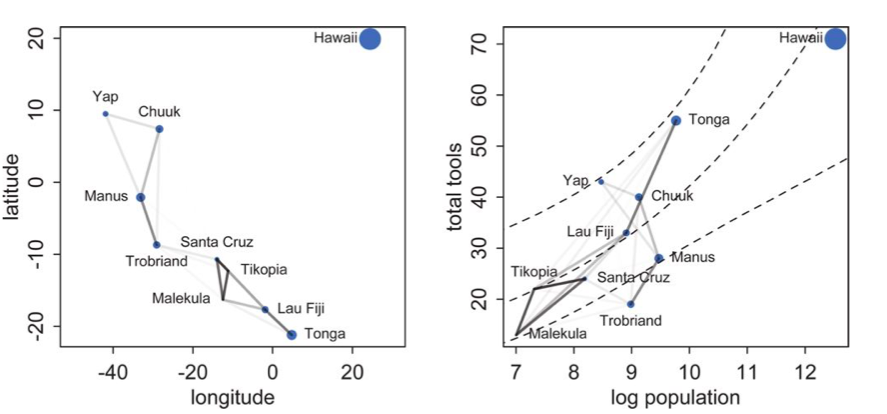
Pacific island societies: geographic locations (left) and total tools vs log population with regression fits (right)

To produce a plot like the one on the right, we calculate the posterior predictives with the correlation free part of the model and then overlay the correlations

from scipy.stats import poisson
def compute_pp_no_corr(lpgrid, idata, contact=0):
    alphatrace = idata.posterior['alpha'].values.flatten()
    betaptrace = idata.posterior['betap'].values.flatten()
    tl=len(alphatrace)
    gl=lpgrid.shape[0]
    lam = np.empty((gl, tl))
    lpgrid = lpgrid - lpgrid.mean()
    for i, v in enumerate(lpgrid):
        temp = alphatrace + betaptrace*lpgrid[i]
        lam[i,:] = poisson.rvs(np.exp(temp))
    return lam

lpgrid = np.linspace(6,13,30)
pp = compute_pp_no_corr(lpgrid, mgctrace)
ppmed = np.median(pp, axis=1)
pphpd = az.hdi(pp.T)

/var/folders/wq/mr3zj9r14dzgjnq9rjx_vqbc0000gn/T/ipykernel_99733/1140317622.py:4: FutureWarning: hdi currently interprets 2d data as (draw, shape) but this will change in a future release to (chain, draw) for coherence with other functions
  pphpd = az.hdi(pp.T)

import itertools
corrs={}
for i, j in itertools.product(range(10), range(10)):
    if i <j:
        corrs[(i,j)]=medcorrij[i,j]
corrs

{(0, 1): np.float64(0.8698352620543791),
 (0, 2): np.float64(0.8112473227705732),
 (0, 3): np.float64(0.00043436736396140004),
 (0, 4): np.float64(0.5149475145540022),
 (0, 5): np.float64(0.1784232683108405),
 (0, 6): np.float64(0.016081624526447357),
 (0, 7): np.float64(0.04062970353128279),
 (0, 8): np.float64(0.23539959071681077),
 (0, 9): np.float64(2.0906899790788574e-06),
 (1, 2): np.float64(0.9154252648017558),
 (1, 3): np.float64(0.0008366129005128546),
 (1, 4): np.float64(0.5139204403538437),
 (1, 5): np.float64(0.18708149396439477),
 (1, 6): np.float64(0.03359131718569693),
 (1, 7): np.float64(0.053427593503310396),
 (1, 8): np.float64(0.20012990301592104),
 (1, 9): np.float64(1.202888923895069e-05),
 (2, 3): np.float64(0.0023184490292404336),
 (2, 4): np.float64(0.3608686936824079),
 (2, 5): np.float64(0.29308742903236046),
 (2, 6): np.float64(0.06359788152183848),
 (2, 7): np.float64(0.10110366922210785),
 (2, 8): np.float64(0.11679105204171875),
 (2, 9): np.float64(7.2267626429193134e-06),
 (3, 4): np.float64(7.5489412116086325e-06),
 (3, 5): np.float64(0.08224827819593294),
 (3, 6): np.float64(0.35861152292486287),
 (3, 7): np.float64(0.33164464636786223),
 (3, 8): np.float64(2.347346485820119e-07),
 (3, 9): np.float64(8.620610481644896e-10),
 (4, 5): np.float64(0.014464210496029285),
 (4, 6): np.float64(0.0013572460520712762),
 (4, 7): np.float64(0.002000507564221195),
 (4, 8): np.float64(0.7531057509569615),
 (4, 9): np.float64(6.197988773284955e-05),
 (5, 6): np.float64(0.25687279780700056),
 (5, 7): np.float64(0.7115819000189696),
 (5, 8): np.float64(0.0020841826197110433),
 (5, 9): np.float64(1.621981972350849e-08),
 (6, 7): np.float64(0.5257538678112668),
 (6, 8): np.float64(8.985523762623615e-05),
 (6, 9): np.float64(1.2616630242151445e-06),
 (7, 8): np.float64(0.00016958954461546093),
 (7, 9): np.float64(1.1170223361457242e-08),
 (8, 9): np.float64(3.3560220950963584e-05)}

with sns.plotting_context('poster'):
    plt.plot(df.logpop, df.total_tools,'o', color="g")
    lpv = df.logpop.values
    ttv = df.total_tools.values
    for a,x,y in zip(df.culture.values, lpv, ttv):
        plt.annotate(a, xy=(x,y))
    for i in range(10):
        for j in range(10):
            if i < j:
                plt.plot([lpv[i],lpv[j]],[ttv[i], ttv[j]],'k', alpha=corrs[(i,j)]/1.)
    plt.plot(lpgrid, ppmed, color="g")
    plt.fill_between(lpgrid, pphpd[:,0], pphpd[:,1], color="g", alpha=0.2, lw=1)
    plt.ylim([10, 75])
    plt.xlim([6.5, 13])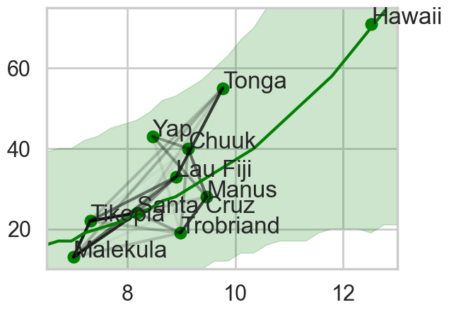

Notice how distance probably pulls Fiji up from the median, and how Manus and Trobriand are below the median but highly correlated. A smaller effect can be seen with the triangle on the left. Of-course, causality is uncertain